How to Decide Which Trendline to Use in Excel

Some options to choose from are moving average linear trendline etc. I have some data that I need to find 50 value for.

How To Add A Trendline In Excel Charts Step By Step Guide Trump Excel

Right-click on the Total line and select Format Data Series.

. Click the Trendline button in the Analysis group. Right-click on any data bar in the chart and select Add Trendline from the menu that appears A to open the Format Trendline task pane B. The maximum R-squared value indicates the best trendline to your data.

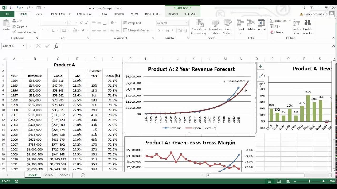
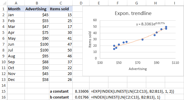
The TREND Function Calculates Y values based on a trendline for given X values. The trendline equation turns out to be y 24585x 13553. The chart consists of the period days as X.

You may choose from several different types of trendlines including linear polynomial exponential and logarithmic. You can calculate moving average manually with your own formulas or have Excel make a trendline for you automatically. Plot your data on a scatter chart rightclick any of the data points then choose Trendline from the resulting dialog.

Use this type To create. The trendline equation will automatically appear on the scatterplot. When youve got got a data set you want to locate the data change trend and forecast them in a graph.

Click the Display R-squared value on chart checkbox D. I like to check the boxes to display both the equation and R-squared statistic. Click the button on the right side of the chart click the arrow next to Trendline and then click More Options.

Note that Excel only displays the Trendline option if you select a chart that has more than one data series without selecting a data series. A sidebar will slide from the right where you can select the trendline of your choice. Choose The Best Trendline.

The trendline is calculated Using the least squares method based on two data series. Select one of the predefined options or click More Trendline Options for a dialog with more detailed settings. For trend lines specifically we recommend using any of the 2D charts.

A drop-down menu appears. To decide the best trendline have a take a observe the R-squared value. Notice how the formula inputs appear TREND function Syntax and inputs.

Now double click on the trendline that has been created on the graph and you will see a Format Trendline options pop up on the right hand side. For a basic trendline indicating the general direction of your data click the radio button to the left of Linear C. On the Format Trendline pane select Moving Average and specify the desired number of periods.

Click More Trendline Options and then in the Trendline Options category under TrendRegression Type click the type of trendline that you want to use. Use a linear trendline for simple data. How can I find a point on a trend line in Excel chart.

Right-click the data series and click Add Trendline. To use the TREND Excel Worksheet Function select a cell and type. After clicking the plus icon found on the upper-right side of the chart click the right arrow beside Trendline and choose More Options from the dropdown list.

Once you choose the category you will get a list of the function displayed as shown in the below screenshot. Activate the Layout tab of the ribbon under Chart Tools. How to Learn More About Excel.

When I use this formula to calculate the difference of max and min pt of trendline 275-419419. Select one of the series in your chart. Then to add a trendline go to Chart Elements or from the green sign at the top right corner of the graph select a linear trendline.

Change the trendline options if the default lines of your data do not match. Lastly get rid of that Total line cluttering up your chart. Right-click on the Total line and Add a trendline will be active.

Use the drop-down menus from the scatter plot diagram and you will see several trendline options. To find the slope of the trendline click the right arrow next to Trendline and click More Options. Choose a chart type.

It is still -0342862273080 which is the same as the result obtained from LOGESTI4U4COLUMNSI4U4-1-1. Click on the Trendline option. In the window that appears on the right side of the screen check the box next to Display Equation on chart.

The Add Trendline dialog box. There are a several different types of trendlines. Choose the insert function and you will get the below dialogue box as shown below.

Using the context menu. Positioned x withinside the equation proven withinside the chart. Specify the number of periods to include in the forecast.

To display a moving average trendline on a chart heres what you need to do. In the Analysis group click Trendline. Click on it and Excel will create the trend line for the total series.

After selecting your chart click on the plus icon to the top right of the chart. Select the category statistically. Choose a TrendRegression type.

Choose the desired type of trendline or click More Trendline Options for other choices make a choice and click Close.

Pin On Lab

Find The Equation Of A Trendline In Excel Youtube

Excel Trendline Types Equations And Formulas